Toward Machine Learning Enhancement of Accelerated Surface Hopping with Scaled Spin–Orbit Couplings

Surface hopping simulations are well suited for ultrafast processes, such as internal conversion through conical intersections, which typically happen within hundreds of femtoseconds. Intersystem crossing (ISC), the transition between states of different spin multiplicity, is a different story. When the spin–orbit couplings (SOCs) driving it are small, ISC can take hundreds of picoseconds, which is far beyond what we can afford to simulate with high-level electronic structure methods.

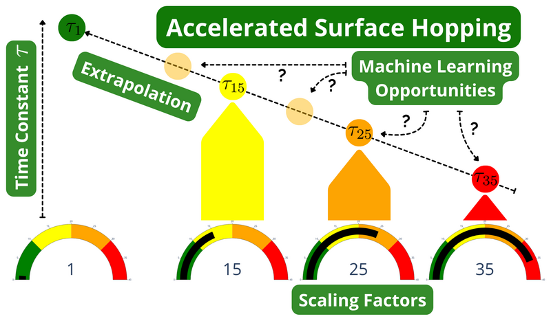
If the goal is only to estimate the time constant, there is a trick: the couplings driving the process can be artificially scaled by a constant $\alpha > 1$,

\[\hat{H}^{\alpha}_{ij} = \alpha \langle \phi_i | \hat{H}_{\mathrm{SO}} | \phi_j \rangle,\]

so that ISC happens within the simulated time window. For a two-state system, Fermi’s golden rule tells us that the rate depends on the square of the coupling, so the time constant scales as

\[\tau_\alpha = \frac{A}{\alpha^2}.\]

Running several ensembles of trajectories with different scaling factors and extrapolating back to $\alpha = 1$ then gives the actual time constant. We refer to this as the Fit1 method; alternatively, fitting a straight line on a log–log scale leaves the exponent as a free parameter (Fit2 method). The catch is that every scaling factor requires its own ensemble of trajectories, so the number of trajectories per ensemble is usually kept small, and the statistical confidence of the result suffers.

In this work, we investigate how reliable such an accelerated scheme is and where machine learning (ML) can help. As a test case, we chose silaethylene (CH₂SiH₂), a small molecule with tiny SOCs and therefore slow transfer to the triplet state.

The reference dynamics were performed at the MR-CISD/SA-CASSCF(2,2) level of theory including S₀, S₁ and T₁, with 200 trajectories for each of the scaling factors 15, 25 and 35. The triplet populations were fitted simultaneously for all scaling factors (multi-curve fitting), and the uncertainties were estimated by bootstrapping. Analyzing ensembles of increasing size showed that at least 100 trajectories per ensemble are needed to obtain a converged time constant, which already makes the accelerated scheme quite expensive.

To replace the expensive reference calculations, we trained a multi-state ANI model for the singlet PESs and a separate ANI model for the triplet. NACs were fitted with kernel ridge regression using the gradient difference descriptor from our previous work, and we extended the rotate-predict-rotate (RPR) approach, together with phase correction, to fit SOCs. Somewhat surprisingly, the best SOC descriptor turned out to be plain Cartesian coordinates rotated into the standard orientation by RPR.

A good test of the ML potentials is the early relaxation of silaethylene, which proceeds either through torsion around the C–Si bond (type T) or through bipyramidalization (type B). Projecting the trajectories onto these two coordinates shows that the ML-driven dynamics reproduce the reference well: 65 % of ML trajectories follow type T and 35 % type B, compared to 72 % and 28 % for MR-CISD.

The S₁ decay is in excellent agreement with the reference, and the ML triplet populations fall within the 95% confidence interval of the MR-CISD data for all scaling factors:

However, the extrapolation turned out to be very sensitive to the fitted time constants. With Fit1, the reference gives 434 ± 106 ps, while ML gives 316 ± 67 ps. The discrepancy comes mainly from the largest scaling factor, which amplifies the errors of the ML models. We therefore recommend a hybrid approach: run reference trajectories with the largest scaling factor, and use them to train ML models that are then employed for the smaller ones.

We also found that the most promising use of ML is not adding more scaling factors, but making each ensemble larger. With 500 ML trajectories per scaling factor, the bootstrapping errors shrink substantially, giving 212 ± 25 ps (Fit1) and 127 ± 170 ps (Fit2).

For detailed information, check out the preprint: (Martinka et al., 2026). The ML part of this work was carried out in MLatom.

References

2026