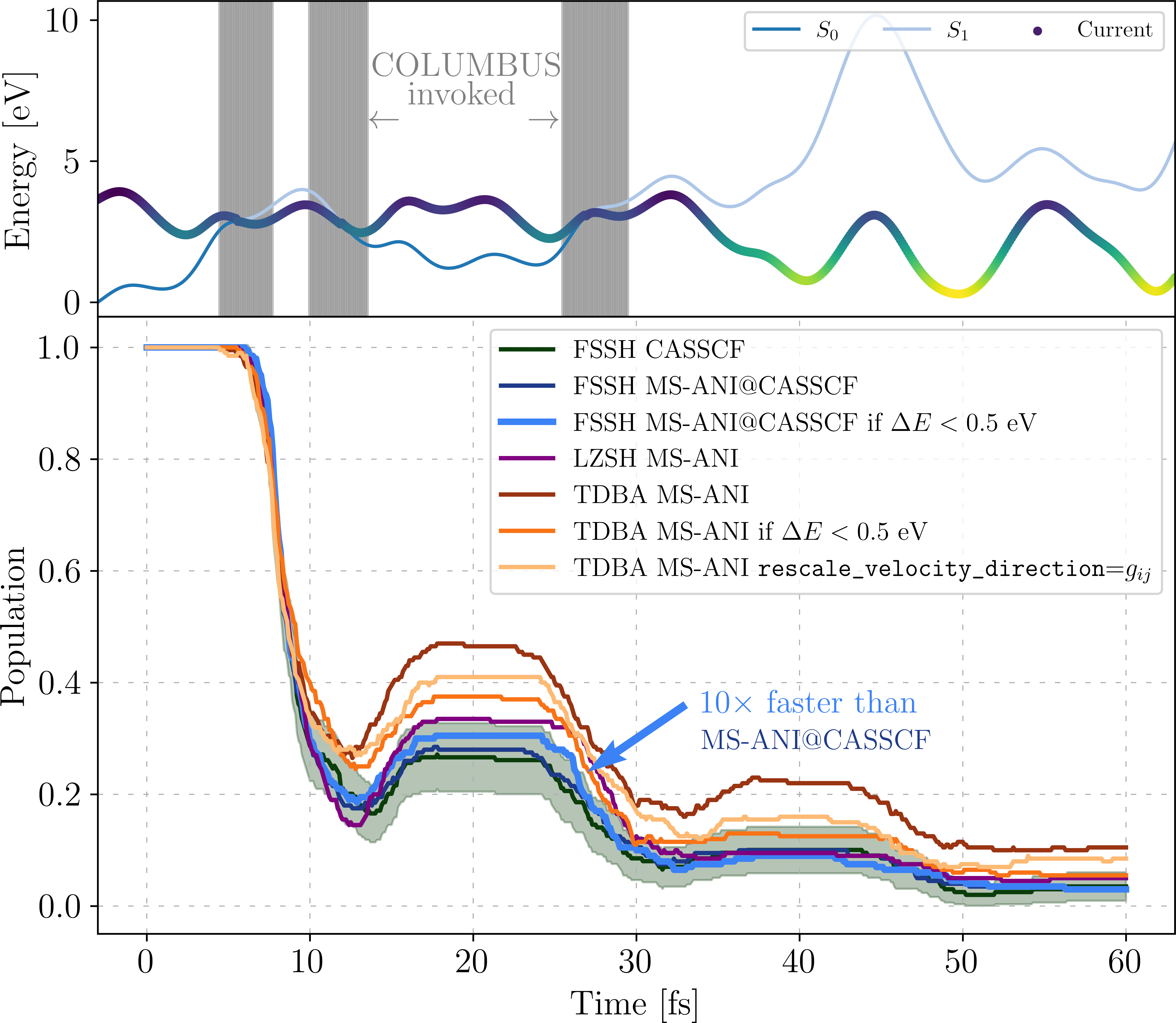
Flexible Framework for Surface Hopping: From Hybrid Schemes for Machine Learning to Benchmarkable Nonadiabatic Dynamics

Surface hopping is a family of simulation techniques that combines quantum description (i.e., solving time-independent Schrödinger equation) with a classical one (integrating Newton’s equations of motion). The evolution of a nucleat wave-packet on excited-state potential energy surfaces (PESs) is approximated by an ensemble of classical trajectories propagating on a single PES, with the possiblity to “hop” between different surfaces. In this way, surface hopping schemes aim to describe photochemical relaxation through conical intersection. In this work, we present a flexible platform for performing such simulations while incorporating machine learning (ML) models, offering several practical advantages.

First, we implemented Tully’s Fewest Switches Surface Hopping (FSSH) scheme together with the time-dependent Baeck-An (TDBA) approach. These implementations are now part of the MLatom package, which can be imported as a Python module. This allows users to conveniently combine diffeent quantum-chemical methods or ML models within a Python workflow. This is achieved by defining custom models with Python classes:

class mlmodels():
    def __init__(self, energy_model, nac_model):
        self.e_model = energy_model
        self.nac_model = nac_model
    
    def predict(self,molecule=None, nstates=2, current_state=0, calculate_energy=True, 
                calculate_energy_gradients=True, calculate_nacv=True):
        molecule.electronic_states = [molecule.copy() for ii in range(nstates)]
        
        # MS-ANI energy + gradient
        self.e_model.predict(molecule=molecule, nstates=nstates, current_state=current_state, calculate_energy=calculate_energy, calculate_energy_gradients=calculate_energy_gradients)
        
        # Columbus NACs
        dE = molecule.electronic_states[1].energy - molecule.electronic_states[0].energy
        if dE * ml.constants.Hartree2eV < 0.5:
            self.nac_model.predict(molecule=molecule, nstates=nstates, current_state=current_state, calculate_energy=False, calculate_energy_gradients=False, calculate_nacv=True)
        else:
            molecule.nacv = np.zeros((nstates,nstates,*molecule.get_xyz_coordinates().shape))

This class example includes a condition that checks wheter energy difference is smaller than 0.5 eV, which significantly reduces the computational cost. Surface hopping can also be performed using only with quantum-chemical methods, provided they supply PESs, gradients and nonadiabatic couplings. Once the input files are prepared, simulations can be executed using the following code snippet:

import mlatom as ml

# Load initial condition
init_cond = ml.data.molecule.load('ic.json', format='json')

# Load MNDO
mndo = ml.models.methods(method='ODM2', read_keywords_from_file='mndokw')

# Run trajectory
dyn = ml.namd.surface_hopping_md(
    model=mndo,
    molecule=init_cond,
    time_step=0.5,
    time_step_tdse=0.025, # not needed for LZSH
    maximum_propagation_time=200,
    hopping_algorithm='FSSH', # 'TDBA' or 'LZSH'
    decoherence_model='SDM', # not needed for LZSH
    rescale_velocity_direction='nacv',
    # or 'gradient difference' or 'momentum'
    nstates=4,
    initial_state=3)

# Save trajectory in H5MD format to disk
dyn.molecular_trajectory.dump('traj.h5', format='h5md')

MLatom provides a wide range of interfaces to both quantum-chemical methods and ML models. Consequently, even when NACs are unavailable, so-called curvature-driven schemes can be employed. These either estimate hopping probability (as in Landau-Zener surface hopping, LZSH) or approximate time-derivative couplings (as in TDBA) based on the curvature of the PESs.

The resulting trajectories can be stored in the binary H5MD format and analyzed using built-in tools. This accelerate development and benchmarking. This following code snippet demonstrates how to load a trajectory and call the plot_trajs() function to analyze it by plotting selected geometrical parameters along with other electronic properties:

import mlatom as ml

traj = ml.data.molecular_trajectory()
traj.load('traj.h5', format='h5md')

ml.namd.plot_trajs(
    trajectories=[traj],
    geom_params=[[0, 1], [0, 1, 4], [3, 1, 0, 5]],
    show_tdc=False,
    only_energy_params=False,
    filename=None
    )

The resulting plot is shown below. Individual subplots can be selected to closely inspect regions of interest.

For detailed information, check out the paper: (Martinka et al., 2025) or GitHub repository associated with this work: FSSH-in-MLatom. All simulations were carried out in MLatom.